
Today we are looking at the Barnes–Hut algorithm, the trick behind most gravity simulations of star clusters and galaxies. I wrote one in Python (compiled with Numba, otherwise we would be here all day), tested it against the exact answer, and checked whether it really is as fast as people say.
The problem with direct summation
Consider \(N\) particles with masses \(m_j\) at positions \(\mathbf r_j\). The acceleration of particle \(i\) is
\[\mathbf a_i = \sum_{j \neq i} \frac{G m_j \left(\mathbf r_j - \mathbf r_i\right)}{\left(\lvert\mathbf r_j - \mathbf r_i\rvert^2 + \epsilon^2\right)^{3/2}},\]where \(\epsilon\) is a small softening length that stops the force blowing up when two particles get very close. Computing this sum for every particle is called direct summation. It is exact (up to rounding), but every particle needs every other particle.
Proof that direct summation is \(O(N^2)\)
The pair \((i, j)\) contributes to \(\mathbf a_i\), and by Newton’s third law the same term, with the opposite sign and \(m_i\) instead of \(m_j\), contributes to \(\mathbf a_j\). So we only need each pair once, and there are
\[\binom{N}{2} = \frac{N(N-1)}{2}\]pairs. Each pair costs the same fixed amount of work (a few subtractions and multiplications, a square root and a division), whatever \(N\) is. The total cost is therefore \(c\,N(N-1)/2\) for some constant \(c\), which is bounded above and below by multiples of \(N^2\). Doubling \(N\) quadruples the work, and nothing clever can be done about it as long as we insist on computing every pair.
On my laptop (one core of an Apple M4 Pro) one force evaluation takes 2.8 s for 50,000 particles and 11.4 s for 100,000. A million particles would take about 19 minutes, and a simulation needs thousands of these evaluations. So we need something better!
The idea of Barnes and Hut
Notice that a distant group of stars pulls on us almost exactly like a single star with the group’s total mass, sitting at the group’s centre of mass. Barnes and Hut (1986) turned this into an algorithm.
- Put all particles in one cube. Split it into 8 smaller cubes (cells), split every cell that still contains more than one particle into 8 again, and so on, until each cell holds at most one particle. This is an octree (in 2D, a quadtree).
- For every cell, store its total mass \(M\) and its centre of mass \(\mathbf R\).
- To find the force on particle \(i\), start at the biggest cell and walk down the tree. For a cell of side \(s\) whose centre of mass is a distance \(d\) from the particle:
- if \(s/d < \theta\), use the whole cell as one point of mass \(M\) at \(\mathbf R\);
- otherwise open the cell and look at its (up to 8) children.
A cell with a single particle is used directly, and a cell that contains particle \(i\) itself is always opened. Salmon and Warren (1994) showed that the plain \(s/d < \theta\) rule can give large errors in unlucky cases, and this extra rule avoids the worst of them.
The parameter \(\theta\) is the opening angle: \(s/d\) is roughly the angle the cell takes up in the sky, seen from the particle. With \(\theta = 0\) every cell gets opened and we are back to direct summation (only slower, because of the tree). A larger \(\theta\) means fewer and bigger cells, so it is faster but less accurate.
The picture below shows this in 2D for 400 particles. The starred particle needs 36 cells and 20 single particles, so 56 interactions instead of 399. Notice that the cells it uses get bigger the further away they are.
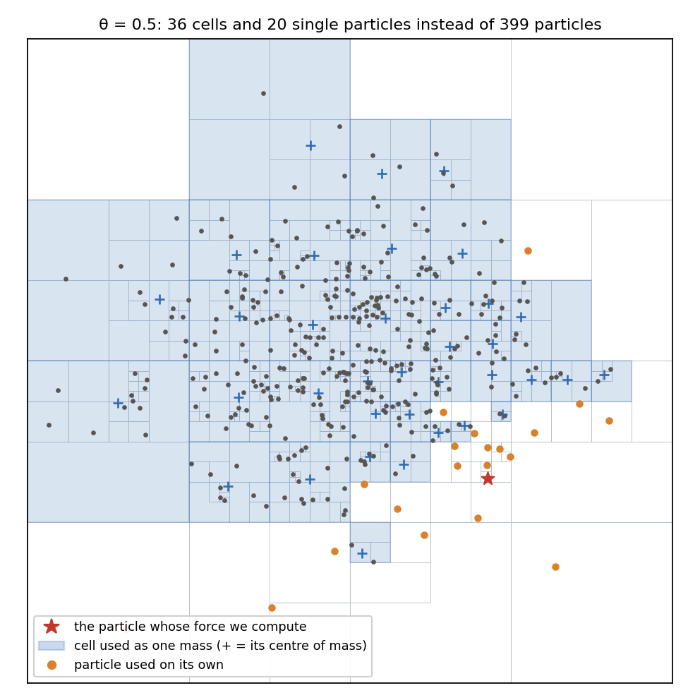
The centre of mass is the right point to put the mass at. If we expand the potential of a cell in powers of \(s/d\) about its centre of mass, the dipole term vanishes (that is exactly what the centre of mass is!). So the first error term is the quadrupole, and using one cell instead of its particles is wrong by roughly \((s/d)^2 < \theta^2\) times that cell’s own pull.
Proof that Barnes–Hut is \(O(N \log N)\)
This one needs an assumption, and I think the assumption is the interesting part. Let \(L\) be the side of the first cube, so a cell on level \(\ell\) of the tree has side \(L/2^{\ell}\) (the first cube is level 0), and let \(D\) be the deepest level.
Step 1: how deep the tree is
A cell is only split if it holds at least two particles, and two particles in a cell of side \(s\) are at most \(\sqrt{3}\,s\) apart. So if the closest two particles are \(d_\text{min}\) apart, no cell smaller than \(d_\text{min}/\sqrt3\) is ever split, and
\[D \le \log_2 \frac{\sqrt{3}\,L}{d_\text{min}} + 1.\]For \(N\) random points in a cube there are about \(N^2/2\) pairs, and a given pair is closer than \(r\) with probability proportional to \(r^3\), so the closest pair is about \(N^{-2/3}L\) apart. Then \(D \approx \tfrac{2}{3}\log_2 N\) plus a constant. For a million random points that is 13.3, and the deepest level of my tree is 14.
Step 2: building the tree
Every particle sits in exactly one cell on each level. Sorting the particles into cells, and adding up the masses and centres of mass, therefore costs a fixed amount per particle per level, so \(O(ND)\) in total.
Step 3: walking the tree
Fix a particle at \(\mathbf x\) and look at one level, where the cells have side \(s\). We only look at a cell on this level if its parent (side \(2s\)) was opened. That happens either because \(2s \ge \theta d\), so the parent’s centre of mass is within \(2s/\theta\) of \(\mathbf x\), or because the parent contains \(\mathbf x\). Every point of the parent is within \(2\sqrt3\,s\) of its centre of mass, so in both cases the whole parent lies inside a ball of radius
\[R = 2s\left(\frac{1}{\theta} + \sqrt{3}\right)\]around \(\mathbf x\). Cells on the same level do not overlap, so at most
\[\frac{\tfrac{4}{3}\pi R^3}{(2s)^3} = \frac{4\pi}{3}\left(\frac{1}{\theta} + \sqrt{3}\right)^3\]parents can be opened, and each has at most 8 children. So on every level we look at no more than
\[C(\theta) = \frac{32\pi}{3}\left(\frac{1}{\theta} + \sqrt{3}\right)^3\]cells. The important thing is that this depends neither on \(s\) nor on \(N\)! Adding up the levels, one particle costs at most \(C(\theta)\,(D+1)\) interactions, and all of them together at most \(N\,C(\theta)\,(D+1)\).
Putting it together
With \(D \approx \tfrac{2}{3}\log_2 N\), building the tree costs \(O(N \log N)\) and walking it costs \(O(N \log N)\) for any fixed \(\theta > 0\) (for small \(\theta\) the constant grows like \(\theta^{-3}\)). So one force evaluation costs \(O(N \log N)\).
The bound is generous: for \(\theta = 0.5\) it allows 1,742 cells per level, while my code needed about 2,100 interactions per particle in total for a million particles in a tree 17 levels deep.
When it fails
The proof needs \(D\) to grow like \(\log N\). This is true for random points, and for realistic star clusters, but not in general. Put particle \(k\) at \(x = 2^{-k}\) on a line: every split separates only one particle from the rest, the tree has \(N\) levels, and building it costs about \(N^2/2\). So “\(O(N \log N)\)” really means “\(O(N \log N)\) unless the particles are absurdly clustered”. Also \(C(\theta)\) blows up as \(\theta \to 0\), which is just the statement that \(\theta = 0\) is direct summation again.
Testing it
The set-up:
- A Plummer sphere, a standard model of a star cluster with a dense core: total mass 1, scale length 1, \(G = 1\), positions drawn with a fixed random seed. For the scaling test, also points spread uniformly in a cube.
- The same softening \(\epsilon = 0.01\) for both methods, so direct summation is the exact answer the tree code should reproduce.
- Cells use their total mass at the centre of mass only (no quadrupole), and every leaf holds one particle.
- Everything runs on one core, so the times measure the algorithm and not how many cores my laptop has.
Accuracy and run time against θ
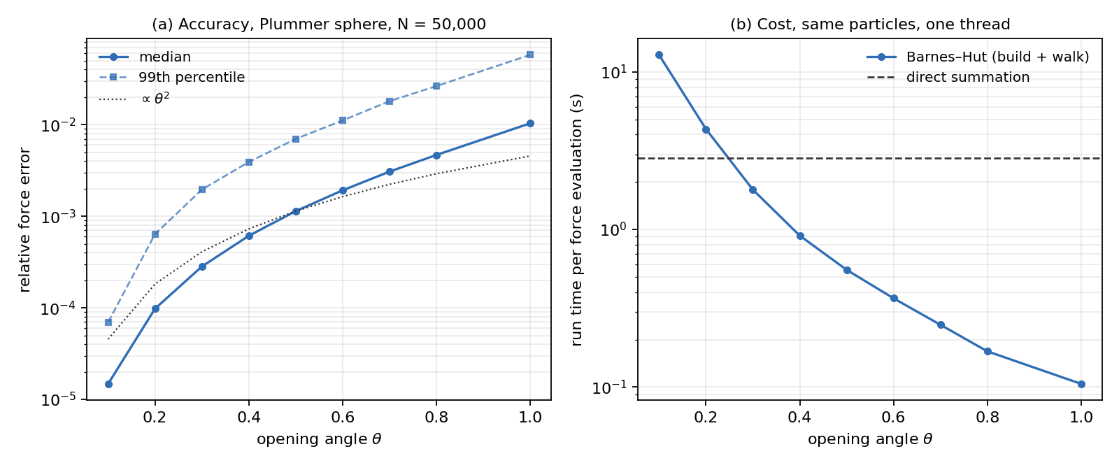
For 50,000 particles I compared the tree force on every particle with the direct sum, using the relative error \(\lvert\mathbf a_\text{tree} - \mathbf a_\text{direct}\rvert / \lvert\mathbf a_\text{direct}\rvert\).
| \(\theta\) | median error | 99th percentile | interactions per particle | run time (s) | speed-up |
|---|---|---|---|---|---|
| 0.1 | 0.0015% | 0.0070% | 24,144 | 12.8 | 0.2× |
| 0.3 | 0.028% | 0.20% | 4,524 | 1.79 | 1.6× |
| 0.5 | 0.11% | 0.70% | 1,514 | 0.55 | 5.1× |
| 0.7 | 0.31% | 1.8% | 685 | 0.25 | 11.4× |
| 1.0 | 1.0% | 5.8% | 319 | 0.11 | 27× |
| direct | exact | exact | 25,000 pairs | 2.83 | 1× |
A few things to notice:
- The error grows a bit faster than \(\theta^2\): between \(\theta = 0.2\) and \(0.8\) the median goes like \(\theta^{2.8}\). I think this is because a larger \(\theta\) does two things at once: every cell is approximated more roughly, and more of the total force comes from cells instead of single particles.
- A small \(\theta\) is pointless at this size. At \(\theta = 0.1\) the tree does about as many interactions per particle (24,144) as direct summation does pairs per particle (25,000, thanks to Newton’s third law), and each of its interactions costs more because of the walk. It breaks even at about \(\theta = 0.25\).
- The worst particles are much worse than the median: at \(\theta = 0.5\) the worst one is off by 3%. The 50 worst sit in the core of the cluster (median distance 0.13 from the centre, against 1.3 for all particles). There the pulls from all sides nearly cancel, so the net force is small, and their absolute errors are also about seven times larger than typical.
Run time against N
| \(N\) | direct (s) | Barnes–Hut (s) | interactions per particle |
|---|---|---|---|
| 1,000 | 0.001 | 0.003 | 363 |
| 10,000 | 0.113 | 0.077 | 1,015 |
| 100,000 | 11.4 | 1.24 | 1,685 |
| 1,000,000 | about 1,140 (19 min, extrapolated) | 21.1 | 2,083 |
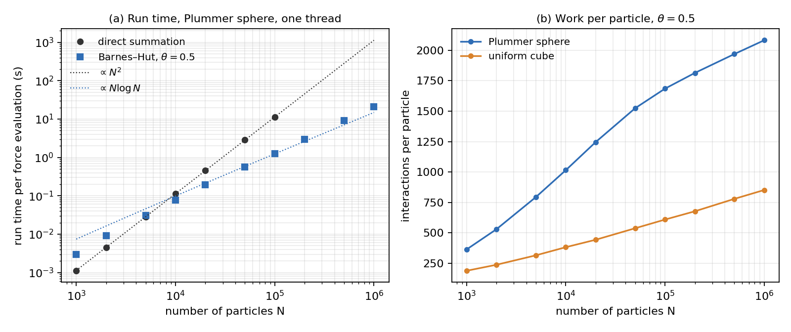
- Direct summation follows \(N^2\) exactly: the slope on the log-log plot is 2.00.
- Below somewhere between 5,000 and 10,000 particles direct summation wins (a simple double loop is hard to beat). At a million particles the tree is about 54 times faster.
- Every time \(N\) is multiplied by 10, the interactions per particle go up by a roughly constant amount, which is exactly what \(\log N\) growth looks like: about 224 more per factor of 10 for the uniform cube. For the Plummer sphere the growth even slows down a little at the largest \(N\).
- The run time of the tree grows with a log-log slope of 1.21, a bit more than \(N \log N\) predicts (about 1.1 in this range). The extra comes from memory, not from the algorithm: the time per interaction rises from 7.5 ns at \(N = 10^4\) to 10 ns at \(N = 10^6\), because the tree no longer fits in the processor’s cache. So the algorithm is \(N \log N\), but the computer is not quite!
Is this verifiable?
Yes, and that was the point of setting it up like this. From the strongest check to the weakest:
- The accuracy is measured against the exact answer for the same particles, so the error table is not an estimate.
- The interaction counts depend only on the particle positions, and those come from a fixed random seed. Anyone who runs the code gets exactly the same counts on any computer. They are also the quantity the proof is about, and they grow like \(\log N\). The proof’s estimate of the depth checks out too: \(\tfrac23\log_2 10^6 \approx 13.3\), against 14 levels in the tree.
- The run times depend on the computer. They confirm \(N^2\) for direct summation exactly, and \(N \log N\) for the tree up to the memory effect above.
Conclusion
Direct summation costs \(N(N-1)/2\) pair interactions. It is exact, and for fewer than a few thousand particles it is also the fastest. Barnes–Hut costs \(O(N \log N)\), as long as the particles are not absurdly clustered, in exchange for a small error that \(\theta\) controls. An opening angle of 0.5 to 0.7 is a sensible choice: a median error of 0.1–0.3%, and a speed-up that keeps growing with \(N\).
Two things would make it better that I did not do here: storing the quadrupole moment of every cell (more accurate for the same \(\theta\)), and the fast multipole method of Greengard and Rokhlin (1987), which brings the cost down to \(O(N)\).
References
- J. Barnes and P. Hut, “A hierarchical O(N log N) force-calculation algorithm”, Nature 324, 446–449 (1986).
- L. Hernquist, “Performance characteristics of tree codes”, Astrophysical Journal Supplement Series 64, 715–734 (1987).
- J. K. Salmon and M. S. Warren, “Skeletons from the treecode closet”, Journal of Computational Physics 111, 136–155 (1994).
- L. Greengard and V. Rokhlin, “A fast algorithm for particle simulations”, Journal of Computational Physics 73, 325–348 (1987).
- H. C. Plummer, “On the problem of distribution in globular star clusters”, Monthly Notices of the Royal Astronomical Society 71, 460–470 (1911).
- S. J. Aarseth, M. Hénon and R. Wielen, “A comparison of numerical methods for the study of star cluster dynamics”, Astronomy and Astrophysics 37, 183–187 (1974).
Filed under Astrophysics, Numerical Methods, Python.