In my summer 2025 project at the University of Edinburgh I simulated two-dimensional Kolmogorov flow with JAX-CFD, a fluid solver written at Google Research in JAX. A common alternative for problems like this is Dedalus, a general framework for spectral methods that is widely used in fluid dynamics and astrophysics. This page runs both on the same problem and compares them: against an exact solution, against linear stability theory, in chaotic flow at Re = 40 and in turbulent flow at Re = 2000. It ends with what each code is good at.
The results of the project itself are not on this page. Everything here was computed in October 2026 for this comparison.
1Kolmogorov flow
Fluid fills a square box of side \(2\pi\) that is periodic in both directions, and a body force pushes it one way in some horizontal bands and the other way in others:
\[\frac{\partial \mathbf u}{\partial t} + (\mathbf u\cdot\nabla)\mathbf u = -\nabla p + \frac{1}{Re}\nabla^2\mathbf u + \sin(4y)\,\hat{\mathbf x}, \qquad \nabla\cdot\mathbf u = 0.\]Kolmogorov proposed this flow around 1959 as a simple setting for studying the transition to turbulence. For every Reynolds number \(Re\) it has an exact steady solution, the laminar flow
\[\mathbf u = \frac{Re}{16}\,\sin(4y)\,\hat{\mathbf x},\]in which the force exactly balances viscosity. The energy put in by the force and the energy dissipated by viscosity are then both \(Re/32\) per unit area. Meshalkin and Sinai showed in 1961 that this flow becomes unstable above a critical Reynolds number. In this box the first disturbance to grow has wavelength \(2\pi\) along the flow, and the critical value is \(Re = 9.967\). Further above it the flow becomes chaotic. Chandler and Kerswell studied the chaotic flow at \(Re = 40\) in detail in 2013, finding many unstable periodic solutions embedded in it, and Page and coworkers have since found hundreds more, using JAX-CFD.
2The two codes
JAX-CFD (Kochkov et al., 2021) was written at Google Research to combine fluid simulation with machine learning. It is written in JAX, so the same code runs on CPUs, GPUs and TPUs, is compiled by XLA, and can be differentiated automatically. For periodic boxes it has a pseudo-spectral solver for the vorticity, which is what I used. Dedalus (Burns et al., 2020) is a general framework: you type the equations in as text, choose a basis for each direction, and it builds a spectral solver. It handles walls, discs and spheres as well as periodic boxes, and runs in parallel with MPI.
| JAX-CFD | Dedalus | |
|---|---|---|
| Unknowns, as used here | vorticity | velocity and pressure (I also timed a vorticity version) |
| Nonlinear term | 2/3 rule | 3/2 padding |
| Time step | Crank–Nicolson with five-stage low-storage Runge–Kutta | four-stage implicit–explicit Runge–Kutta (RK443) |
| Hardware | CPU, GPU, TPU | CPU, in parallel with MPI |
| Gradients | automatic, through the whole solver | not built in (version 3.0) |
| Geometry | periodic boxes; a separate finite-volume solver allows walls | Fourier, Chebyshev and other bases: boxes, channels, discs, spheres |
| Equations | a fixed set | almost any equations, typed in as text |
To make the comparison fair, both codes run in double precision on a single CPU thread, on the same grid and from the same initial vorticity. Every diagnostic is computed by one script from the vorticity each code returns, so neither is measured differently.
3An exact solution
The simplest test is the laminar flow itself. Started exactly on it at \(Re = 8\) on a 64 × 64 grid, after 100 time units JAX-CFD has changed the vorticity by \(5\times10^{-14}\) of its size and Dedalus by \(8\times10^{-15}\): both keep it to round-off.
One trap is worth knowing about. By default, JAX-CFD’s kolmogorov_forcing places the force on the faces of the grid cells, half a cell away from the points where the spectral solver stores the vorticity. The force it applies is then \(\sin 4(y + \Delta y/2)\), and the steady state is shifted by half a cell. That does not change the physics, since it only moves the whole flow, but it breaks comparisons with exact solutions and with other codes: started on the laminar flow above, the vorticity drifts by 20 % on a 64 × 64 grid. Passing offsets=((0, 0), (0, 0)), as JAX-CFD’s own ForcedNavierStokes2D does, removes the shift.
4The onset of instability
Below \(Re = 9.967\) a small disturbance of the laminar flow decays, and above it the disturbance grows. Linear theory gives the rate. Writing the disturbance as a sum of waves \(e^{i(\alpha x + m y)}\), the laminar flow couples each \(m\) to \(m \pm 4\), and the growth rate is the largest real part of the eigenvalues of the resulting matrix. I added a disturbance of size \(10^{-7}\) to the laminar flow at \(Re\) = 8, 9, 10, 11 and 12 on a 64 × 64 grid, followed it in each code, and fitted its growth rate once the fastest mode had taken over.
| \(Re\) | Linear theory | JAX-CFD | Dedalus |
|---|---|---|---|
| 8 | −0.07130 | −0.07111 | −0.07130 |
| 9 | −0.03580 | −0.03578 | −0.03580 |
| 10 | +0.00126 | +0.00126 | +0.00126 |
| 11 | +0.04050 | +0.04050 | +0.04050 |
| 12 | +0.08212 | +0.08205 | +0.08205 |
Both codes reproduce the theory to within 0.3 % at every Reynolds number. The largest differences, at \(Re = 8\) and 9, come from the end of the fit, when the disturbance has decayed by a factor of \(e^{12}\) and JAX-CFD’s slightly larger round-off starts to show.
5Chaos at Re = 40
Both codes start from the same state, the laminar flow plus a disturbance with root-mean-square velocity 0.1, on a 128 × 128 grid with time step 0.005, and run for 600 time units. At this Reynolds number the laminar flow is strongly unstable (σ = 2.35), so the disturbance takes over within a few time units and the flow becomes chaotic. Most of the time the flow is fairly quiet, with dissipation about a tenth of the laminar value, but now and then it bursts and the dissipation more than doubles.
Averaged from \(t = 100\) to 600, as a mean ± standard error (standard deviation in brackets):
| Divided by the laminar value | JAX-CFD | Dedalus |
|---|---|---|
| Energy \(E/E_{\text{lam}}\) | 0.444 ± 0.003 (0.023) | 0.435 ± 0.005 (0.026) |
| Dissipation \(D/D_{\text{lam}}\) | 0.095 ± 0.005 (0.031) | 0.101 ± 0.009 (0.045) |
| Energy input \(I/I_{\text{lam}}\) | 0.095 ± 0.005 (0.033) | 0.101 ± 0.009 (0.046) |
The standard errors come from splitting each run into 20 blocks of 25 time units. The averages agree within them: the energies differ by 1.6 standard errors and the dissipations by 0.6. In each code the average energy input equals the average dissipation, as it must when the energy is not drifting. The errors are a few per cent because 500 time units hold only a few bursts. The Dedalus run happened to spend 35 time units in strong bursts (dissipation above 0.2 of the laminar value), the JAX-CFD run only 10, which is why its fluctuations are larger.
Why do two correct codes, started from the same state, end up with different flows? They discretise the equations differently (section 2), so after one time unit their vorticity fields already differ by about \(10^{-7}\) of their size. In a chaotic flow a small difference grows exponentially. Figure 4 shows it growing by a factor of \(e\) about every 15 time units until, by \(t \approx 140\), the two runs are unrelated. Even round-off error alone would do this, given a few hundred more time units. Chaotic simulations can therefore be compared only through their statistics, not snapshot by snapshot.
At \(Re = 40\) the spectra lie close together on this scale, though not exactly: they differ by up to 70 % at \(k = 2\) and 3 and by up to a factor of 8 far out in the tail, which the strongest bursts dominate. These differences are sampling, not a disagreement between the codes: the two halves of the Dedalus run differ from each other by more, by a factor of 4.7 at \(k = 2\). The spectrum has fallen by 14 decades at \(k = 40\), so a 128 × 128 grid resolves this flow with plenty to spare.
6Turbulence at Re = 2000
At \(Re = 2000\) the flow is turbulent, with filaments of vorticity far thinner than the forcing bands, so I used a 512 × 512 grid and a time step of 0.001. A statistically steady state at this Reynolds number takes thousands of time units to form, because energy collects in the largest scales and viscosity removes it only slowly. On one CPU thread, 2000 time units would take Dedalus about a week. Instead, both codes start from the same random field, with root-mean-square velocity 1 and typical wavenumber 6, and run for 10 time units.
Dedalus did not finish: with the same fixed time step as JAX-CFD it became unstable at \(t = 9.7\), once the fastest velocity had grown above 6. This is a property of the schemes, not a bug. An explicit step for advection is stable only while \(\Delta t\, u_{\max}\, k_{\max}\) stays below a limit set by the scheme. That limit is 1.57 for the explicit part of Dedalus’s RK443 and 3.34 for JAX-CFD’s five-stage scheme. Dedalus’s nonlinear term also reaches wavenumber 256 instead of 170, because it pads rather than truncating. At \(t = 9.5\) the product was 1.62 for Dedalus, just past its limit, and 1.08 for JAX-CFD. In normal use Dedalus would shrink its step as the flow sped up, using its CFL tool. The upshot is that on this problem JAX-CFD can take steps about three times longer. I compare the two runs up to \(t = 9.5\), where both are clean: the energy and dissipation agree to within \(10^{-4}\) until the moment Dedalus fails, and its spectrum shows no build-up before it.
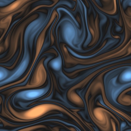
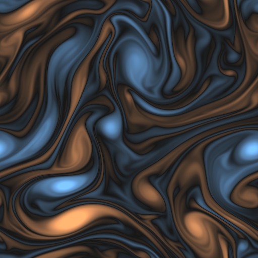
Both runs start from the same random field. After 9.5 time units they differ by 3 % of the size of the field, too little to see.
Up to \(t = 9.5\) the total energy agrees to \(10^{-4}\), and the spectra agree to 0.1 % up to \(k = 100\) and to 3 % near the cutoff (switch Figure 5 to \(Re = 2000\)). The fields differ more than at \(Re = 40\) at the start, by \(5\times10^{-4}\) already at \(t = 0.5\). A little over half of that comes from wavenumbers above 170, which JAX-CFD’s 2/3 rule leaves out of the nonlinear term and Dedalus keeps. That part stays at about \(2\times10^{-3}\), while the rest grows as the chaos amplifies it. The spectrum falls by about nine decades between the forcing scale and the cutoff, so the 512 × 512 grid resolves this window, though without much margin.
7Cost
Time per step on one thread of an Apple M4 Pro, in double precision, as the best of three timings with nothing else running (JAX 0.4.30 with JAX-CFD 0.2.1, Dedalus 3.0.5):
| Grid | JAX-CFD | Dedalus, velocity and pressure | Dedalus, vorticity |
|---|---|---|---|
| 128 × 128 | 1.4 ms | 13.9 ms | 8.7 ms |
| 256 × 256 | 4.7 ms | 67 ms | 39 ms |
| 512 × 512 | 20 ms | 336 ms | 192 ms |
JAX-CFD is 10 to 17 times faster than Dedalus in velocity and pressure, and 6 to 10 times faster than Dedalus solving the same vorticity equation, and the gap widens with the grid. It manages this while evaluating the nonlinear term five times per step to Dedalus’s four. Part of the difference is dealiasing: with 3/2 padding the transforms act on a grid 2.25 times larger than the 2/3 rule needs. The rest is how the work is organised. JAX-CFD compiles the whole step into one program for this one equation, while Dedalus is built to handle any equations and bases, which costs time on a problem this simple. The longer stable step at high \(Re\) (section 6) widens the gap further. In the 600-time-unit runs at \(Re = 40\), JAX-CFD took 3 minutes and Dedalus 31.
I did not test the cases each code is designed for at scale: GPUs, where JAX-CFD runs fastest, and many cores, where Dedalus splits one simulation across processes with MPI.
8Gradients through the solver
The strongest reason to use JAX-CFD is not speed. Because the whole solver is written in JAX, it can be differentiated: JAX can return the gradient of any quantity computed from the flow with respect to the initial state, or to parameters such as \(Re\), by running the computation backwards (reverse-mode automatic differentiation).
As a test, I took a chaotic state at \(Re = 40\) on a 64 × 64 grid, ran it forward 1000 steps (5 time units), and asked for the gradient of the final energy with respect to all 4096 values of the initial vorticity. Along a random direction, this gradient agrees with a central finite difference to \(3\times10^{-9}\), and computing it took 2.2 times as long as the forward run alone.
| Finite-difference step \(h\) | Finite difference | Relative difference from the gradient |
|---|---|---|
| \(10^{-2}\) | −0.051716351 | \(3.8\times10^{-5}\) |
| \(10^{-3}\) | −0.051718278 | \(3.8\times10^{-7}\) |
| \(10^{-4}\) | −0.051718298 | \(3.4\times10^{-9}\) |
| \(10^{-5}\) | −0.051718298 | \(5.1\times10^{-9}\) |
| automatic differentiation | −0.051718298 |
With finite differences, the same gradient would need two runs for each of the 4096 directions. This is what makes gradient-based methods practical: finding unstable periodic orbits by minimising how far a flow is from repeating itself, as Page and coworkers did, fitting initial states to observations, or training a neural network inside the solver. Dedalus 3.0, the version I used, does not differentiate its solvers automatically; a gradient there needs an adjoint solver, written and checked separately.
9Which to use
Both codes are correct: they agree with the exact solution, with linear theory and with each other’s statistics. The choice depends on the problem.
JAX-CFD is the better tool for flows in periodic boxes when you need many or long runs, GPUs, gradients, or a coupling to machine learning. On one CPU thread it was 6 to 17 times faster per step here, and it tolerated a longer step.
Dedalus is the better tool when the problem is not a periodic box or not a standard equation: walls, discs or spheres, rotation, stratification, magnetic fields or extra fields, all typed in as equations. It scales across many cores with MPI. Writing the equations out as text also makes some mistakes harder, such as the misplaced forcing in section 3.
For my project, a periodic box with many long runs, JAX-CFD was the natural choice, and its gradients make the optimisation methods used in this field available directly.
10References
- K. J. Burns, G. M. Vasil, J. S. Oishi, D. Lecoanet and B. P. Brown, “Dedalus: A flexible framework for numerical simulations with spectral methods,” Phys. Rev. Research 2, 023068 (2020).
- M. H. Carpenter and C. A. Kennedy, “Fourth-order 2N-storage Runge–Kutta schemes,” NASA Technical Memorandum 109112 (1994).
- G. J. Chandler and R. R. Kerswell, “Invariant recurrent solutions embedded in a turbulent two-dimensional Kolmogorov flow,” J. Fluid Mech. 722, 554 (2013).
- D. Kochkov, J. A. Smith, A. Alieva, Q. Wang, M. P. Brenner and S. Hoyer, “Machine learning–accelerated computational fluid dynamics,” Proc. Natl. Acad. Sci. 118, e2101784118 (2021).
- L. D. Meshalkin and Ya. G. Sinai, “Investigation of the stability of a stationary solution of a system of equations for the plane movement of an incompressible viscous liquid,” J. Appl. Math. Mech. 25, 1700 (1961).
- J. Page, P. Norgaard, M. P. Brenner and R. R. Kerswell, “Recurrent flow patterns as a basis for two-dimensional turbulence: Predicting statistics from structures,” Proc. Natl. Acad. Sci. 121, e2320007121 (2024).