
Part 4 of 11 of the research log of my 2024 summer project on the three-body problem, at the University of Edinburgh, supervised by Prof. Jenni Smillie.
Previous: Ellipses and the Two-Body Problem
Next: Understanding and Visualising the Shape Sphere
This post introduces the problem of two fixed centres, also known as Euler’s three-body problem: a small body moving under the gravity of two masses held fixed in place. Unlike the general three-body problem, it is integrable.
Set-up
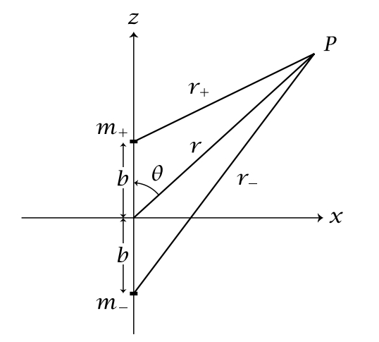
The two fixed masses \(m_\pm\) sit on the \(z\)-axis at \(z = \pm b\), and the third body moves in the \(x\)–\(z\) plane.
Simulation
To simulate the problem, I held two of the masses fixed and let the third move freely:
The Lagrangian
The natural coordinates are prolate spheroidal coordinates \((R, \sigma)\), which play the role of polar coordinates but with two foci:
\[x = \pm \sqrt{R^2-b^2}\, \sin \sigma, \qquad z = R \cos \sigma .\]Writing \(\mathbf{r}(R, \sigma) = (x, z)\), the partial derivatives are
\[\begin{aligned} \frac{\partial x}{\partial R} &= \pm \frac{R \sin \sigma}{\sqrt{R^2 - b^2}}, & \frac{\partial z}{\partial R} &= \cos \sigma, \\ \frac{\partial x}{\partial \sigma} &= \pm \sqrt{R^2 - b^2}\, \cos \sigma, & \frac{\partial z}{\partial \sigma} &= -R \sin \sigma, \end{aligned}\]so (taking the \(+\) sign)
\[\begin{aligned} \mathbf{r}_R &= \frac{\partial \mathbf{r}}{\partial R} = \begin{pmatrix} \frac{R \sin \sigma}{\sqrt{R^2 - b^2}} \\ \cos \sigma \end{pmatrix}, \\ \mathbf{r}_\sigma &= \frac{\partial \mathbf{r}}{\partial \sigma} = \begin{pmatrix} \sqrt{R^2 - b^2}\, \cos \sigma \\ -R \sin \sigma \end{pmatrix} . \end{aligned}\]The metric components \(g_{RR}= \mathbf{r}_R \cdot \mathbf{r}_R\), \(g_{R\sigma} = \mathbf{r}_R\cdot\mathbf{r}_\sigma\) and \(g_{\sigma\sigma} = \mathbf{r}_\sigma\cdot\mathbf{r}_\sigma\) come out as
\[\begin{aligned} g_{RR}&=\frac{R^2-b^2 \cos ^2 \sigma}{R^2-b^2}, \qquad g_{R \sigma}=0, \\ g_{\sigma \sigma}&=R^2-b^2 \cos ^2 \sigma . \end{aligned}\]The distances to the two centres are \(R \mp b\cos\sigma\), so the potential energy per unit mass is
\[\begin{gathered} V=-\mu\, \frac{R+\beta b \cos \sigma}{R^2-b^2 \cos ^2 \sigma}, \\ \mu = G(m_+ + m_-), \qquad \beta=\frac{m_{+}-m_{-}}{m_{+}+m_{-}} . \end{gathered}\]The Lagrangian per unit mass is therefore
\[\begin{aligned} \mathcal{L} = T-V &=\frac{1}{2}\, \frac{R^2-b^2 \cos ^2 \sigma}{R^2-b^2}\, \dot{R}^2 \\ &\quad+\frac{1}{2}\left(R^2-b^2 \cos ^2 \sigma\right) \dot{\sigma}^2 \\ &\quad+\mu\, \frac{R+\beta b \cos \sigma}{R^2-b^2 \cos ^2 \sigma} . \end{aligned}\]Jacobi elliptic functions
The equations of motion separate in these coordinates. Following the book, the equation for \(S = \cos\sigma\) reduces, after a change of independent variable from \(t\) to \(f\), to the form
\[S^{\prime 2}=\left(1-S^2\right)\left(1-k^2 S^2\right),\]whose solution is
\[S=\operatorname{sn}(f+\omega \mid k).\]Here \(\operatorname{sn}\) is one of the Jacobi elliptic functions. Trigonometric functions are defined with reference to a circle, and the Jacobi elliptic functions generalise them to other conic sections, in particular the ellipse.
To verify the solution, use
\[\frac{d}{du} \operatorname{sn}(u \mid k) = \operatorname{cn}(u \mid k) \operatorname{dn}(u \mid k)\]together with the identities
\[\begin{aligned} \operatorname{sn}^2(u \mid k) + \operatorname{cn}^2(u \mid k) &= 1, \\ \operatorname{dn}^2(u \mid k) + k^2 \operatorname{sn}^2(u \mid k) &= 1 . \end{aligned}\]With \(u = f + \omega\), these give \(\operatorname{cn}^2 u = 1 - S^2\) and \(\operatorname{dn}^2 u = 1 - k^2 S^2\), so
\[S'^2 = \operatorname{cn}^2(u \mid k)\, \operatorname{dn}^2(u \mid k) = (1 - S^2)(1 - k^2 S^2) .\]Part 11 compares this solution with a simulated orbit.
Credits
This post is based on the book Integrable Systems in Celestial Mechanics by Diarmuid Ó’Mathúna. Parts of the material on Jacobi elliptic functions are from Wikipedia.
Revised on 25 October and 11 November 2026. Nothing in the results was wrong. The potential now comes with the definitions of \(\mu\) and \(\beta\), and the modulus is written \(k\) instead of \(k_{01}\). The note on the momentum bug moved to part 2, where the problem is described.
Filed under Classical Mechanics, Research, Three-Body Problem.