
Part 11 of 11 of the research log of my 2024 summer project on the three-body problem, at the University of Edinburgh, supervised by Prof. Jenni Smillie.
This post continues the problem of two fixed centres from part 4 and part 6.
New types of orbits
The run in part 6 started from rest and stayed around one of the two centres, so \(S = \cos\sigma\) covered only part of its range. Giving the body an initial velocity produces two further types of orbit, lemniscate and planetary.
To classify them, we need two constants of motion. With the centres at \((\pm d, 0)\) and masses \(m_1\) and \(m_2\),
\[\begin{aligned} G&=\frac{1}{2}\left(x p_y-y p_x\right)^2+\frac{1}{2} d^2 p_x^2 \\ &\quad+d x\Biggl(\frac{m_1}{\sqrt{(x+d)^2+y^2}} \\ &\qquad-\frac{m_2}{\sqrt{(x-d)^2+y^2}}\Biggr), \\ H&=\frac{1}{2}\left(p_x^2+p_y^2\right) \\ &\quad-\frac{m_1}{\sqrt{(x+d)^2+y^2}}-\frac{m_2}{\sqrt{(x-d)^2+y^2}} . \end{aligned}\]\(H\) is the energy, and \(G\) is the additional constant of motion discovered by Euler, which makes the problem integrable. The mass of the moving body drops out of the equations of motion, so \(p_x\) and \(p_y\) are momenta per unit mass.
The paper Syzygies in the Two Center Problem shows that the values of \(H\) and \(G\) determine the type of orbit: \(S\) (satellite, the type found in part 6), \(L\) (lemniscate) and \(P\) (planetary).

My simulations reproduce all three types:


Why a body released from rest stays on one side
For equal masses, the equation for \(S\) from part 4 can be written with these two constants. Let \(R\) be the mean of the distances to the two centres, so that \(S = x/R\), and let \(f\) be the variable defined by \(df = dt/(R^2 - d^2 S^2)\). Then
\[\left(\frac{dS}{df}\right)^2 = 2G\left(1-S^2\right)\left(1-\frac{H d^2}{G}\, S^2\right).\]A body released from rest has no kinetic terms in \(G\), which leaves \(G = d\,x\,(m_1/r_1 - m_2/r_2)\). This is negative on either side of the line \(x = 0\), because the nearer centre has the larger \(m/r\). With \(G\) and \(H\) both negative, the right-hand side is non-negative only where
\[S^2 \ge \frac{G}{H d^2},\]so \(S\) never reaches zero and the body never crosses to the other side, whatever its energy. That is the satellite orbit of part 6, and it is why starting from rest could not give anything else. As a check, a body released from rest at \((1.6, 1.2)\), with \(d = 1\) and unit masses, has \(G = -0.634\) and \(H = -1.095\). The bound is \(\lvert S\rvert \ge 0.761\), and in the simulation \(S\) stays between 0.761 and 1.
When \(G > 0\) the right-hand side is positive for every \(\lvert S\rvert < 1\), so \(S\) sweeps the whole interval. These are the lemniscate and planetary orbits. They differ in whether \(R\) comes down to \(d\), that is, whether the body passes between the centres.
S follows sn in the right variable
With the new orbits \(S\) covers its full range, but against time it looks irregular:

In 2024 I could not see \(\operatorname{sn}\) in this plot. The reason is that the solution is a function of \(f\) and not of \(t\). The two are related by \(dt = (R^2 - d^2 S^2)\, df\), so a given step in \(f\) takes little time when the body is close to the centres and a long time when it is far away. Against \(f\) the oscillation is exactly periodic, and it is the Jacobi function
\[S = \operatorname{sn}\left(\sqrt{2G}\, f + \omega \,\middle|\, k\right), \qquad k^2 = \frac{H d^2}{G} .\]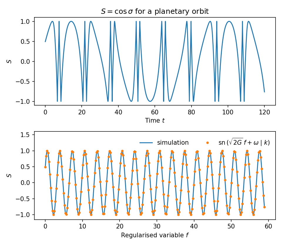
For this orbit \(k^2 = -0.324\). A bound orbit with \(G > 0\) always has \(k^2 < 0\), an imaginary modulus, for which \(\operatorname{sn}\) is still real and periodic.
Next steps
- Map out which initial conditions lead to each of \(S\), \(L\) and \(P\).
- Extend the analysis to unequal fixed masses, where the equation for \(S\) gains a term linear in \(S\).
The comparison of simulated orbits with \(G\) and \(H\) was later written up as a short paper, An Analysis of the Restricted Euler Problem Using Symplectic Integrators.
Credits
This post draws on Syzygies in the Two Center Problem and the book Integrable Systems in Celestial Mechanics by Diarmuid Ó’Mathúna.
Revised on 25 October and 11 November 2026. The original quoted values of the book’s parameter \(e\) for the three orbits (2.5, 0.98 and 1.08). They came from a bug in the code that computed them and are removed. The original also left two things open: why \(S\) did not look like \(\operatorname{sn}\), and whether the mass of the moving body matters. Both are now answered in the text. The equation for \(S\) in terms of \(G\) and \(H\), the argument about bodies released from rest and the last figure were added in the second revision.
Filed under Classical Mechanics, Research, Three-Body Problem.