Problem of Two Fixed Centres (Part II)

Summer research 2024: the three-body problem · Part 6 of 11

A weekly research log from my summer project at the University of Edinburgh, supervised by Prof. Jenni Smillie.

← Understanding and Visualising the Shape Sphere  ·  Sundman's Power Series Solution to the Three-Body Problem (Part I) →

This post continues the problem of two fixed centres, introduced in part 4, by converting my simulated trajectories into the coordinates in which the theory is written.

From Cartesian to prolate spheroidal coordinates

Recall the prolate spheroidal coordinates \((R, \sigma)\), with the centres at distance \(b\) from the origin and \(\sigma \in [0, \pi]\):

\[x= \pm \sqrt{R^2-b^2}\, \sin \sigma, \qquad z=R \cos \sigma .\]

The sign of \(x\) is carried by the \(\pm\), so it is enough to consider \(x \geq 0\). Take \(b = 1\).

Substituting \(R = z/\cos\sigma\) into the first equation and squaring,

\[\begin{aligned} x^2 &= \sin^2 \sigma \left(\frac{z^2}{\cos^2 \sigma} - 1\right) = \frac{(z^2 - \cos^2 \sigma)\sin^2 \sigma}{\cos^2 \sigma} \\ &= \frac{(z^2 - 1 + \sin^2 \sigma)\sin^2 \sigma}{1 - \sin^2 \sigma}, \end{aligned}\]

which rearranges to

\[x^2 = \sin^2 \sigma \left(x^2 + z^2 - 1 + \sin^2 \sigma\right).\]

(This step divides by \(\cos\sigma\), so it fails on the line \(z = 0\), which has to be handled separately.) Setting \(u=\sin^2\sigma\) gives a quadratic,

\[u^2+(x^2+z^2-1)\,u-x^2=0,\]

whose non-negative root is

\[u = \frac{-(x^2 + z^2 - 1) + \sqrt{(x^2 + z^2 - 1)^2 + 4x^2}}{2} .\]

Then \(\sigma_1 = \arcsin\sqrt{u}\) lies in \([0, \pi/2]\). Since \(z = R\cos\sigma\) with \(R \ge 0\), this is the correct angle when \(z \ge 0\); when \(z<0\) the angle lies in \((\pi/2, \pi]\), and we take \(\sigma = \pi - \sigma_1\):

\[\sigma = \begin{cases} \sigma_1, & z \ge 0, \\ \pi - \sigma_1, & z < 0. \end{cases}\]

Given \(\sigma\), \(R = z/\cos\sigma\) follows immediately (or \(R = \sqrt{x^2/\sin^2\sigma + b^2}\) near \(z = 0\)).

Results

For this trajectory:

the coordinate \(R\) evolves as

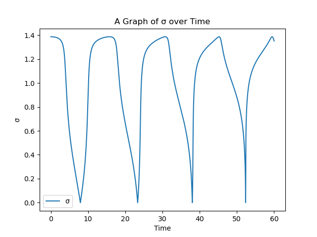
the angle \(\sigma\) as

and \(S = \cos\sigma\) as

Issues

The moving body never crosses the saddle point of the potential between the two centres (analogous to a Lagrange point), so it stays around only one of the fixed masses. This disagrees with the theory: \(S\) should behave like the Jacobi function \(\operatorname{sn}\), so \(\sigma\) should sweep through its whole range, whereas here it covers only part of it.

Two assumptions may be responsible:

• I implemented the fixed centres by holding two bodies in place; it may be better to give them very large masses instead.
• The test body starts at rest. A larger initial velocity may let it pass the saddle point.

Progress

Matching the constants in the book to the parameters in my code has been the hardest part so far. Over the next weeks I plan to study Sundman’s series, which I expect to be computationally very demanding.

Credits

This post is based on the book Integrable Systems in Celestial Mechanics by Diarmuid Ó’Mathúna.

Changes on 25 October 2026

What was wrong. The discussion of which branch of \(\arcsin\) to take described \(\sigma\) in the range \(\pi/2 < \sigma < 3\pi/2\), but in these coordinates \(\sigma\) only runs from 0 to \(\pi\).

What changed. The rule is now stated directly: \(\sigma = \sigma_1\) when \(z \ge 0\) and \(\sigma = \pi - \sigma_1\) when \(z < 0\).