Linear Regression using OLS and SGD Methods in Python

Linear Regression is very widely used in data analysis. Many people run the analysis in Excel, but do you know you can read the data from an Excel file and plot the analysis (as well as calculate many very useful metrics) in Python?

Methods to fit a Linear Model

In Python, there are many ways to fit a Linear Model. Below, we will mainly focus on the OLS (Ordinary Least Square) Method, which will minimize the sum of the squares of the differences. Afterwards, we will be using rhe SGDRegressor (Linear model fitted by minimizing a regularized empirical loss with SGD (Stochastic Gradient Descent Algorithm)). More can be found here.

How to know if your linear regression model is accurate?

• \(R^2\) Score
  • It represents the proportion of the variance in the dependent variable that can be explained by the independent variables used in the model. (See below for more theoretical details)
  • Scikit-Learn Function: sklearn.metrics.r2_score
• Mean Absolute Error (MAE)
  • The average of the absolute errors between the predicted values and the actual values.
  • Scikit-Learn Function: sklearn.metrics.mean_absolute_error
• Mean Squared Error (MSE) (Mainly used for SGD)
  • The average of the squared errors between the predicted values and the actual values
  • Scikit-Learn Function: sklearn.metrics.mean_squared_error
• Root Mean Squared Error (RMSE)
  • The square root of the MSE. It provides error in the same unit as the dependent variable.
• Residual Plots
  • A good fit is indicated by residuals randomly scattered around zero without any discernible pattern.

We will mainly use \(R^2\), MSE, and MAE in the analysis below.

Running Linear Regression on World Population Data

Given the World Population Data we can try to find and plot a linear trend in the data.

We start by storing the data in an Excel file and then read it into Python using the Pandas library. This allows us to handle and manipulate the data easily. The data consists of years (independent variable) and the world population (dependent variable).

OLS Method

We use \(80 \%\) of the data for training our model, which means this portion of the data is used to “learn” the relationship between the years and the world population (by finding \(m\) and \(c\) in \(y=mx+c\) that minimises the sum of square residues). The remaining \(20 \%\)is used to test and validate the model’s accuracy.

SGD Method

For the SGD method, we would first need to scale the independent variable (the years) to ensure fairness in the optimization process. We then use the SGDRegressor function to minimize the MSE by iteratively moving towards the minimum value, with a maximum iteration of \(1000\). After \(1000\) iterations, the best fit line which minimises the MSE will be plotted.

By following these steps, we can attempt to find and visualize the linear trend in the world population data using either the OLS or SGD regression methods.

Results

OLS Method

• MSE: 503030576553090.75
• \(R^2\): 0.9997738328468143
• MAE: 17666518.47913985

SGD Method

• MSE: 454359657773408.56
• \(R^2\): 0.9997335657388569
• MAE: 16986193.058504555

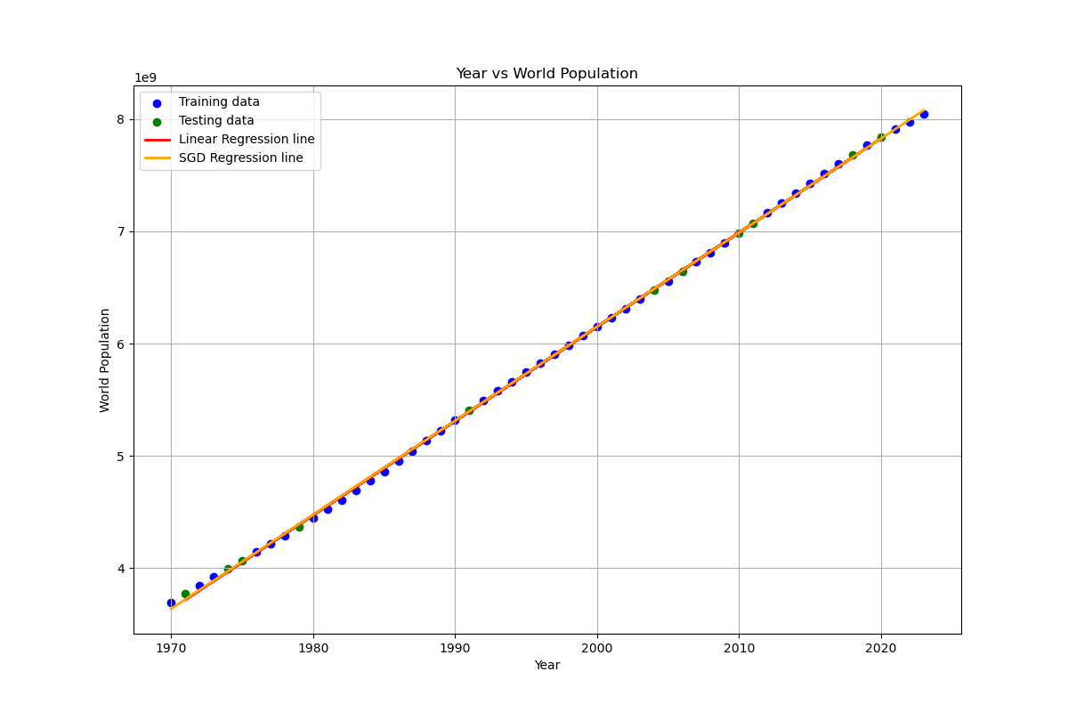
The difference is very minimal, but the SGD Method is slightly more accurate!

Here is an image of the fit (Red line for OLS Method, Orange Line for SGD Method, but they almost overlap!):

Code for Population Regression

import matplotlib.pyplot as plt
import numpy as np
import pandas as pd
from sklearn.model_selection import train_test_split
from sklearn.linear_model import LinearRegression, SGDRegressor
from sklearn.metrics import mean_squared_error, r2_score, mean_absolute_error
from sklearn.preprocessing import StandardScaler

# Read the data from the Excel file
df = pd.read_excel('world_population_data.xlsx')

# Convert the data to numpy arrays and reshape
years = df['Year'].to_numpy()[:, np.newaxis]
populations = df['World Population'].to_numpy()[:, np.newaxis]

# Split the data into training and testing sets
years_train, years_test, populations_train, populations_test = train_test_split(
    years, populations, test_size=0.2, random_state=42
)

# Initialize and train the Linear Regression model
regr = LinearRegression()
regr.fit(years_train, populations_train)
populations_pred_lr = regr.predict(years_test)

# Calculate metrics for Linear Regression model
mse_lr = mean_squared_error(populations_test, populations_pred_lr)
r2_lr = r2_score(populations_test, populations_pred_lr)
mae_lr = mean_absolute_error(populations_test, populations_pred_lr)

# Standardize the data for SGDRegressor
scaler = StandardScaler()
years_scaled = scaler.fit_transform(years)

# Initialize and train the SGDRegressor
sgd_reg = SGDRegressor(max_iter=1000, tol=1e-3, penalty='l2', alpha=0.0001, random_state=42)
sgd_reg.fit(years_scaled, populations.ravel())
populations_pred_sgd = sgd_reg.predict(years_scaled)

# Calculate metrics for SGDRegressor model (using all data since we didn't split)
mse_sgd = mean_squared_error(populations, populations_pred_sgd)
r2_sgd = r2_score(populations, populations_pred_sgd)
mae_sgd = mean_absolute_error(populations, populations_pred_sgd)

# Print the metrics
print(f"Linear Regression - MSE: {mse_lr}, R²: {r2_lr}, MAE: {mae_lr}\n")
print(f"SGD Regressor - MSE: {mse_sgd}, R²: {r2_sgd}, MAE: {mae_sgd}")

# Plot the results
plt.figure(figsize=(12, 8))

# Plot the training and testing data
plt.scatter(years_train, populations_train, color='blue', label='Training data')
plt.scatter(years_test, populations_test, color='green', label='Testing data')

# Plot the regression lines
plt.plot(years_test, populations_pred_lr, color='red', linewidth=2, label='Linear Regression line')
plt.plot(years, populations_pred_sgd, color='orange', linewidth=2, label='SGD Regression line')

# Labels and title
plt.xlabel('Year')
plt.ylabel('World Population')
plt.title('Year vs World Population')
plt.legend()
plt.grid(True)

# Show the plot
plt.show()