Leo Chow - Relativity

This set of notes is from Leo Chow, a student in the University of Hong Kong, on special relativity. I have met him in person and he has personally permitted me to upload his blog in my website.

Relativity

Let’s take a look at the Lorentz factor:

\[\gamma_v=\frac{1}{\sqrt{1-\frac{v^2}{c^2}}}\]

On the right hand side is a recurring structure in the theory of relativity - it shows up in formulae frequently enough for people to give it a symbol. The structure at first sight may seem quite unmotivated apart from students getting some Pythagorean feel from the squares and square root, and judging from the negativie sign that the denominator sould say something about shrinking.

This blog is an attempt to add more intuition to the anatomy of \(\gamma\), and would suggest that an interpretation focusing on velocities instead of length allows for a more succinct and intuitive form for the Lorentz factor:

\[\gamma_v=\sec\theta\]

• Precursors: Speed of light and transverse distances are constant between inertial frames

• Product: Time dilation factor is \(\frac{1}{\sqrt{1-\frac{v^2}{c^2}}}\)

(We are just revisiting the derivation of time dilation here, feel free to skip it)

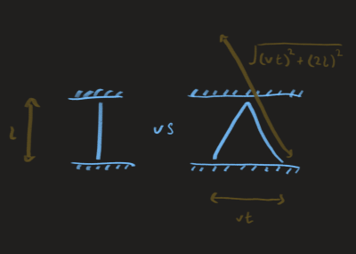
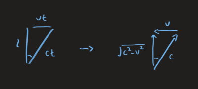
Consider a photon bouncing between two mirrors separated by \(l\), for an inertail frame moving at speed \(v\) perpendicular to \(l\), express the period of light clock \(t\) in terms of the period in the clock \(t\) in terms of the period in the clock’s rest frame \(t_o\).

To keep things short, here’s a usual derivation of the time dilation factor:

\[\begin{gather} ct=\sqrt{(2l)^2+(vt)^2} \\ (ct)^2-(vt)^2=(2l)^2 \\ t^2=\frac{(2l)^2}{c^2-v^2}=\frac{(ct_o)^2}{c^2-v^2} \\ t=\frac{ct_o}{\sqrt{c^2-v^2}}=\frac{t_o}{\sqrt{1-(\frac{v^2}{c^2})^2}} \end{gather}\]

and we get our time dilation factor \(\gamma\). (In line one, the LHS follows from the speed of light being constant, the RHS follows from tranverse distance being constant)

With this, we can already interpret why Lorentz factor is the reverse projection factor \(\sec\theta\). All that the above proof is saying is that relative velocity adds to distance but not speed of light, so motion takes longer. That distance, being perpendicular to \(v\), is scaled up by the reverse projection factor \(\sec\theta\) - which can be expressed in terms of \(c\) and \(v\), by considering a similar triangle with sides consisting of velocities instead of lengths - so Lorentz factor is simply that.

Noticing the similar triangle constructed with velocities instead, you probably get a hint that there exist an alternative view of the derivation using velocities instead of distances.

\[(\text{length, reverse projection)} \rightarrow \text{(velocity, projection)}\]

Let’s look at the following incorrect way of deriving the same thing:

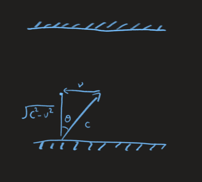
To the observer, the clock is moving with speed \(v\), a component of \(c\) is used to provide the horizontal velocity to keep up with the clock, thus only the vertical component of \(c\) is used to transverse the distance \(2l\). (The vertical component is just \(c\) reduced by \(v\), i.e. \(\sqrt{c^2-v^2}\), or for a more speakable and conceptual formula, just read it as “the projection of \(c\) onto \(l\)” i.e. \(c\cos{\theta}\). We therefore obtain \(t\) much more elegantly,

\[t=\frac{2l}{\sqrt{c^2-v^2}}=\frac{t_o}{\sqrt{1-\frac{v^2}{c^2}}}\]

It seems to be a better derivation than method one, except it is wrong. (Well, if our method here was correct, why would literally all textbooks choose to use the more clumsy version of the derivation instead…)

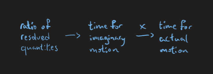
We resolve the velocity vertically, resolved the length of path vertically, take their ratio to get a time quantity, then somehow claim that this time quantity is indeed the time for the original motion (1). Where did we get wrong?

For this, we would need to take a step back and ask the question: why can we resolve a motion into components? We can certainly resolve a motion, but what does that ratio of resolved quantities means? It is the duration in an imaginary situation where a photon is moving along a length of \(2l\) at speed \(\sqrt{c^2-v^2}\), but photons always travel at \(c\).

But why did we get the correct result?

When we do things this way, we are actually doing a Galilean transformation implicitly, to say we resolved the velocity vertically and claim that the time of journey remain unchanged is actually to shift into the light clock’s rest frame in a Galilean way. It still gives the correct Lorentz factor because Galilean transformation is an incorrect way to shift reference frames. So in some sense we are still in the observer’s frame, giving us the correct dilated time.

Alternatively, you can say that the result is correct because we did a forbidden move twice, first is to reduce \(c\) (spatial part of Galilean transform), second is to say that the durations are equal (temporal part of Galilean transform).

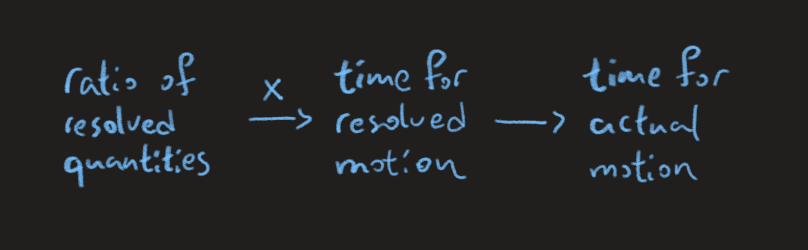
The problem is not with resolving components, the problem is with jumping to the conclusion that the time quantity obtained as the ratio of resolved quantities equals the time for the unresolved motion. To conclude that they are equal, we need to do a Galilean transformation, which is forbidden. Note the characteristic \(t'=t\) here

We would bump into similar problem if we avoid the above picture and consider instead the time for vertical position to reach its final value. (The difference is subtle but it’s there, a subtle attachment is made which, we will see, forces a detachment at another place.)

At (1) we may be tempted to think that the time for the vertical position to reach its final value is of course the time for the position vector to reach its final value and so our method should be justified, just don’t interpret the physical meaning of the ratio as in the above.

This is in fact true by definition. We can expect the event of position vector \(\bold{p}\) reaching its final value to be defined by all its components \(p_i\) reaching each final value. But then we get another problem, how we came to conclude that duration for vertically resolved motion \(t_y\) is given by the ratio \(\frac{L_y}{v_y}\), where \(L=2l\), when all we actually know is :

\(t=\frac{\sqrt{{L_y}^2+{L_x}^2}}{\sqrt{{v_y}^2+{v_x}^2}}\) (path length over speed).

See , now that we detached our “vertical time” \(t_y\) from the imaginary motion along \(L\), we need a Galilean transformation into the orginal frame to conclude \(t_y=\frac{L_y}{v_y}\), which already feels circular if not wrong.

\[t_y=t=\frac{\sqrt{{L_y}^2+{L_x}^2}}{\sqrt{{v_y}^2+{v_x}^2}}=\frac{\sqrt{{L_y}^2+{L_x}^2-(v_xt)^2}}{\sqrt{{v_y}^2+{v_x}^2-{v_x}^2}}=\frac{L_y}{v_y}\]

The first step follows from the temporal part of the transformation \((t'=t)\),the third step follows from the spatial part \((x'=x-{v_x}t)\)

We took a forbidden move to step into an imaginary realm, calculate \(t\) there, then bring it back to the real world by doing another forbidden move. This is reminiscent of a recurring theme in math, consider well known examples like differentiation under the integral sign, Laplace transform or even matrix diagonalization (transform to eigen basis, do the transformation easily, return to original basis). They all have the look \(Q \wedge Q^{-1}\).

In fact, even when people refuse to use the forbidden move, they are still implicitly doing it when rearranging the expression in method one to group \(t\) together on one side. It is just a matter of whether you are willing to interpret the algebra beyond the numerical values into physical meanings. Compare the two methods, you can see that they are just playing with the same triangle:

only that the triangle in method II is formed by thinking about how perspective shift subtract from velocities, instead of how it adds to displacement, the sides are scaled down by \(t\), \(t\) therefore only shows up in one of the side lengths, making the formula for Lorentz factor immediately obvious.

By pretending that we could just project the velocity downwards onto the transverse, we immediately get the projection factor \({\gamma}^{-1}\) as \(\frac{\sqrt{c^2-v^2}}{c}\), because it is \(c\) reduced by \(v\) over original \(c\).

Side Notes:

\[\gamma_v=\left[1-\left(\frac{c}{v}\right)^2 \right]^{-\frac{1}{2}}\]

Rewriting it just for fun, we can see how it is almost \(\frac{c}{v}\), its as though we constructed it by starting with the proportion \(\frac{c}{v}\), uncoiling it at layer ^-2, then just shove the shell \(s(x)=1-x\) into it as a wedge that stop the layers from collapsing back onto itself. It can act as a wedge because \(s\) does not commute with ^-2.

I mention this because I was planning to in some future write about how a small change in the form of a differential equation relates to the resulting change in the form of its solution, you can see that this is some kind of meta-differentiation, and in that discussion this method of reconstruction will show up again. As a sneak peak for now, consider the solution of the logistic growth,

\[P=\frac{K}{(\frac{K-P_o}{P_o})e^{-rt}+1}\]

motivated by how similar the coefficient of the exponential looks compared to the larger structure outside, we flatten the expression to:

\[k(((k^{-1}P_o-1)e^{rt})^{-1}+1)^{-1}\]

and see that if the \(s(x)=x-1\) shell could commute with the \(e^{rt}\) and the ^-1 shell, the whole structure would collapse onto itself back to the exponential growth. An extra factor of \((1-\frac{P}{K})\) in the DE somehow opens up the solution \(P_oe^{rt}\) at various layers - \(KK^{-1}\), ^(-1) ^(-1), -1+1 — then swap the order of operations in such a way that cannot be undone. The result is a knot.

\[\begin{gather} P_oe^{rt} \\ KK^{-1}P_oe^{rt} \\ K\left[(K^{-1}P_oe^{rt})^{-1}\right]^{-1} \\ K\left[(K^{-1}P_oe^{rt})^{-1}-1+1\right]^{-1} \\ K\left\{\left[(K^{-1}P_o-1)e^{rt}\right]^{-1}+1\right\}^{-1}\\ P=\frac{K}{(KP_o^{-1}-1)e^{-rt}+1} \end{gather}\]