Classifying and Finding New Possible Orbits (Part I)

This is the tenth post on my summer research about three-body problems. Today we are discussing my search of possible new planet orbits. This is intended to be part I of the series.

This is my previous post about the proof of Figure 8 orbit if you have missed it.

Motivation and Initialization

If you have followed my series closely you will know my code can return the plots and trajectories of the 3 bodies given initial conditions. It has also been shown that trajectories are highly sensitive to initial conditions.

Now we have two variables \(a\) and \(b\). Assume all three planets have unit mass, i.e. \(M_1 = M_2 = M_3 =1\) and the gravitational constant is unity, i.e. \(G=1\).

Also, the first planet has a starting position of \((-1,0)\) and a starting velocity \((a,b)\), the second planet has a starting position of \((0,0)\) and a starting velocity of \((a,b)\), and the third planet has a starting position of \((1,0)\) and a starting velocity of \((-2a, -2b)\).

Now we vary \(a\) and \(b\) both from \(0\) to \(1\), with a \(0.01\) step, what will happen?

Obviously some orbits will be periodic. As an example, the Figure-8 Orbit will be plotted here, with \((a,b) =(0.35, 0.53)\). Whereas in some orbits two (or even three) of the planets will collide.

In my code, I run the simulation for \(50000\) steps, with a timestep of \(0.001\). If the sum of displacements of the three particles exceed a certain limit (before the \(50000\) steps are reached), it will return False. Otherwise, it will return True and the corresponding point will be plotted in a scatter plot.

Results

The code ran for \(32\) hours.

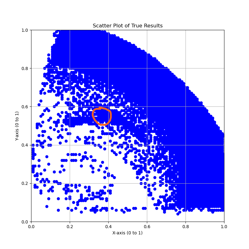
I have circled out the region where the Figure-8 orbit lies. The reader can see immediately that around the circled region, it is more susceptible to a change in \(V_y\) compared to \(V_x\).

This confirms the findings of Ramos.

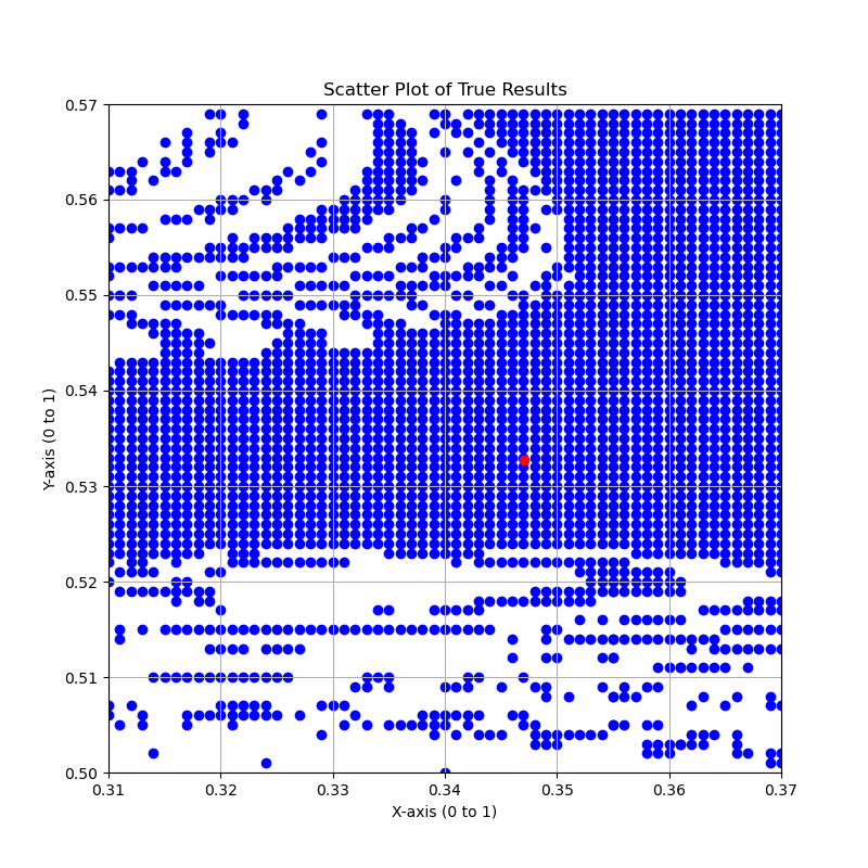
A clearer “zoomed-in” version can be seen below (This ran for around \(15\) hours):

Downsides

The separations allowed is too large. In fact, I think it is impossible to determine an upper bound for the maximum distance between particles.

Let \(E\) be the total energy of the system. Now take \(T=0\). Hence \(E=V\).

Now as \(G=1\) and \(M_1 = M_2 = M_3 = 1\), we have:

\[V = \frac{1}{a} + \frac{1}{b} + \frac{1}{c}\]

Meanwhile \(a\), \(b\), \(c\) should form a triangle. Now assume \(a\) is the longest side. Then, we need:

\(b+c \geq a\).

Now we can pick:

\[V = \frac{1}{\lambda} + \frac{1}{\lambda-b} + \frac{1}{b+0.1}\]

The reader can show that for any \(\lambda\) there exists \(b\) satisfying \(b, \lambda>0\) and \(\lambda \neq b\).

Hence I believe there isn’t an upper bound for \(\lambda\).

Therefore, I was quite unsure of what value of maximum displacement I should pick. In fact, I picked \(20\) as the maximum displacement of any particle from the origin. This is proved to be too large.

Possible Fix using the Return Proximity Function

Using the Return Proximity Function might be a good idea.

\[P(t)=\left|\mathbf{X}(t)-\mathbf{X}_0\right|=\sqrt{\sum_i^3\left[\mathbf{r}_i(t)-\mathbf{r}_i(0)\right]^2+\sum_i^3\left[\mathbf{p}_i(t)\right]^2}\]

A periodic orbit will show oscillations, with a small minimum value (The smaller it is, the closer it is to initial conditions). In the next run, I will choose orbits that has \(P<15\) throughout the simulation and with \(P_{min} (t \neq 0) <0.7\)

Progress

It is quite frustrating that a simulation takes over \(30\) hours to run. The code seems fairly optimised, so I will try to change the timestep from \(0.001\) to \(0.01\), but first I will double check that the accuracy won’t be too compromised.

It is week \(5\) of the project already (out of \(8\)) and I don’t have much progress in terms of original research. I will see what I can do.

Credits

I am inspired by the paper New Families of Periodic Orbits for the Planar Three-Body Problem Computed with High Precision.

I would like to thank Dr Jenni Smillie for her guidance and support duing this project.