Perturbations - Classical Mechanics
Perturbations in Classical Mechanics vs. Quantum Physics
While both classical mechanics and quantum physics employ the term perturbation to denote a small deviation from some reference state, their implementations and outcomes differ significantly.
1. Classical Perturbations: Simple Harmonic Response
A small disturbance of a stable equilibrium in classical mechanics typically induces (possibly damped) simple harmonic motion. Starting from Newton’s second law,
\[F = m\ddot{x},\]a restoring force of the form $F = -\alpha x$ (with $\alpha > 0$) gives
\[-m\ddot{x} = \alpha x \quad\Longrightarrow\quad \ddot{x} + \frac{\alpha}{m}\,x = 0,\]whose solution is sinusoidal with frequency $\omega = \sqrt{\tfrac{\alpha}{m}}$.
2. Central-Force Orbits and Radial Equation
For a particle of mass $m$ under a purely radial force $F_r(r)$, conservation of angular momentum $h = r^2\dot{\theta}$ and Newton’s second law yield:
\[\ddot{r} - \frac{h^2}{r^3} = \frac{F_r(r)}{m}.\]A circular orbit at radius $r = a$ satisfies:
\[0 - \frac{h^2}{a^3} = \frac{F_r(a)}{m},\quad \Longrightarrow\quad F_r(a) = -\frac{m\,h^2}{a^3}.\]3. Small Radial Perturbations of a Circular Orbit
Introduce a tiny radial displacement:
\[r(t) = a + \rho(t),\quad |\rho| \ll a.\]Substitute into the radial equation:
\[\ddot{\rho} - \frac{h^2}{(a + \rho)^3} = \frac{F_r(a + \rho)}{m}.\]Linearize both sides via Taylor expansion to first order in $\rho$:
-
Centrifugal term
\[\frac{1}{(a + \rho)^3} \approx \frac{1}{a^3}\Bigl(1 - 3\frac{\rho}{a}\Bigr).\] -
Radial force
\[F_r(a + \rho) \approx F_r(a) + F_r'(a)\,\rho.\]
Plugging in and cancelling the zeroth-order balance $-h^2/a^3 = F_r(a)/m$ leaves:
\[\ddot{\rho} + \Bigl[\tfrac{3h^2}{a^4} - \tfrac{1}{m}F_r'(a)\Bigr]\rho = 0.\]Define
\[\omega^2 \equiv \tfrac{3h^2}{a^4} - \tfrac{1}{m}F_r'(a).\]Then
\[\ddot{\rho} + \omega^2\,\rho = 0,\]with general solution
\[\rho(t) = A\cos(\omega t + \phi).\]Stability condition: For oscillatory (bounded) motion, $\omega^2 > 0$, i.e.
\[\frac{3h^2}{a^4} > \frac{1}{m}F_r'(a).\]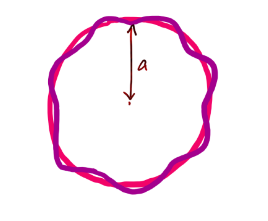
4. Escape Criterion for an Inverse-Square Force
The conserved total energy is
\[E = \tfrac12 m\bigl(\dot r^2 + r^2\dot{\theta}^2\bigr) + V(r), \quad V'(r) = -F_r(r).\]At $t=0$, choose initial conditions
\[\dot r(0) = 0,\quad r_0 = a + \varepsilon,\quad h = r_0^2\dot{\theta}(0),\]so the energy is
\[E = \frac{h^2}{2m\,r_0^2} + V(r_0).\]For an inverse-square law $V(r) = -\frac{k}{r}$ with $h^2 = \tfrac{k a}{m}$, the escape threshold $E = 0$ implies
\[\frac{h^2}{2m\,r_0^2} - \frac{k}{r_0} = 0 \quad\Longrightarrow\quad r_0 = 2a.\]Thus any $r_0 \ge 2a$ (i.e.\ $\varepsilon \ge a$) yields $E \ge 0$ and the particle escapes.
-
Linear (local) stability
Small oscillations around
\(r = a\)
will remain small—nothing “blows up” if
\(|\rho| \ll a.\) -
Escape (global) criterion
If you instead give the particle a large enough “kick” so that
\(r_0 \ge 2a,\)
its total energy becomes non‑negative and it will escape to infinity—even though infinitesimal perturbations are stable.