Image Processing using Python and Convolution Theorem

The use of convolution in image processing is widely discussed. The mathematics and intuition behind is very well described by 3B1B:

Convolution Theorem

Perhaps one of the most important theorems of all:

\[\mathcal{F}[f(t) \ast g(t)]=F(s)G(s)\]

describes a faster way to do large scale convolutions: Fourier Transforming \(f(t)\) into \(F(s)\) and \(g(t)\) into \(G(s)\) first, then applying inverse Fourier Transform to the product of \(F(s)\) and \(G(s)\).

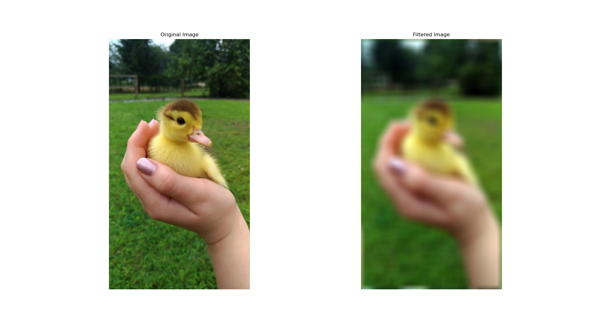
Blurring and Sharpening of Images

I have created a python program where the user can input an arbitary kernel, which will be convolved with images inputted. Source of Image

Using the “Box Blurring Kernel”: (\(50 \times 50\) array filled with ones and normalized)

Using the “Edge Sharpening Kernel”:

\[\begin{bmatrix} -1 & 0 & 1 \\ -2 & 0 & 2 \\ -1 & 0 & 1 \\ \end{bmatrix}\]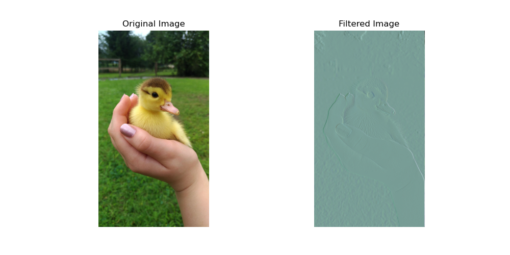

Python Code Demonstration

The steps roughly follow that of the Convolution Theorem. The key is to do it separately for each colour channel, then recombine them at the end.

import numpy as np
import matplotlib.pyplot as plt
import imageio.v2 as imageio
from scipy.fftpack import fftn, ifftn, fftshift

def read_scalars_from_file(filename):
    """
    Reads scalar values from a file and returns them as a list of floats.

    Parameters:
    - filename (str): The name of the file to read.

    Returns:
    - scalars (list): A list of floats representing the scalar values read from the file.
    """
    with open(filename, 'r') as file: 
         for line in file:
            
            lst = line.strip().split()
            
            # map applies float to all the elements in lst
            scalars = list(map(float, lst))
         if len(lst) != 9:
           raise Exception("Enter the values row by row, separating them with spaces. An example is: 1 0 0 0 1 0 0 0 1. Only 3x3 Matrices are supported!")                          
           return None
       
    return scalars

# Print out the Kernel
scalars=read_scalars_from_file('scalars.txt')

def custom_filter():
    """
    Returns:
    - filt (numpy.ndarray): A custom filter represented as a 3x3 numpy array.
     The scalars, a to i, are read from the file as explained above. 
    """
    
    filt = np.array(scalars).reshape((3, 3))
    
    #This is for box blurring

    #filt = np.ones((50, 50)) / 2500  
    return filt


def apply_filter_to_channel(channel, filt):
   pad_height = (channel.shape[0] - filt.shape[0]) // 2
   pad_width = (channel.shape[1] - filt.shape[1]) // 2
   filt_pad = np.pad(filt, ((pad_height, channel.shape[0] - filt.shape[0] - pad_height),
                           (pad_width, channel.shape[1] - filt.shape[1] - pad_width)), mode='constant') 
   
   F = fftn(channel)
   H = fftn(fftshift(filt_pad))  # Shift the padded filter before FFT

   # Multiply in the frequency domain
   G = F * H

   # Perform the inverse Fourier transform and shift
   g = ifftn(G).real

   # Normalize the result for display
   g -= g.min()
   g /= g.max()
   
   return g


image = imageio.imread("duc.jpg")


# Since our image has red, green, blue, they are separatedly convolved with the kernel and recombined at the end
red_channel = image[:, :, 0]
green_channel = image[:, :, 1]
blue_channel = image[:, :, 2]
    
custom_filter=custom_filter()
# Apply the filter to each channel
red_filtered = apply_filter_to_channel(red_channel, custom_filter)
green_filtered = apply_filter_to_channel(green_channel, custom_filter)
blue_filtered = apply_filter_to_channel(blue_channel, custom_filter)
   
# Combine the filtered channels back into a color image
filtered_image = np.stack((red_filtered, green_filtered, blue_filtered), axis=-1)
  
# Plotting the two images side by side for comparison 
fig, axs = plt.subplots(1, 2, figsize=(10, 5))
axs[0].imshow(image)
axs[0].set_title('Original Image')
axs[0].axis('off')
axs[1].imshow(filtered_image)
axs[1].set_title('Filtered Image')
axs[1].axis('off')
plt.show()

Fast Fourier Transform

The astute reader may notice that Fast Fourier Transform (FFT) has been used above. It provides a much faster way to compute Fourier Transforms, with a time complexity of \(O(n \log n)\) instead of \(O(n^2)\).

The most wide used Algorithm is the Cooley–Tukey algorithm. A simplied case is illustrated in my other post.