Understanding and Visualizing the Shape Sphere

This is the fifth post on my summer research about three-body problems. Today we are discussing the shape sphere.

This is my previous post about the problem of two fixed centers if you have missed it.

Simplifying the Three Body Problem through Reduction

Reduction is a method used to simplify the analysis of three body problems by eliminating redundant degrees of freedom.

The three bodies are lying in the Cartesian Plane \(\mathbb{R}^2 \cong \mathbb{C}\). Without “reduction”, the initial configuration space of the system is \(\mathbb{C}^3\), representing the positions of the three masses. To simplify the problem, we use Galilean invariance to fix the center of mass at the origin. This reduces the configuration space to

\[X = \left\{ x = (x_1, x_2, x_3) \in \mathbb{C}^3 \mid \sum_{i=1}^3 x_i = 0 \right\}.\]

By removing the translational degree of freedom, we reduce the dimensionality of the configuration space to \(X\), where \(X \sub \mathbb{C}^3\).

Next, we consider the rotational symmetry of the system. This includes rotation and reflection:

\[R_\theta \cdot (x_1, x_2, x_3) = (e^{i\theta} x_1, e^{i\theta} x_2, e^{i\theta} x_3), \quad S \cdot (x_1, x_2, x_3) = (\bar{x}_1, \bar{x}_2, \bar{x}_3).\]

To further reduce the configuration space, we consider the quotient of \(X\) by the rotation group \(SO(2)\), which represents all possible rotations in the plane.

The reduced configuration space, after factoring out translations and rotations, is homeomorphic to \(\mathbb{R}^3\). This space represents the set of oriented similarity classes of triangles. This space is known as the shape space.

Mathematical Details

First we define the Jacobi Map:

\[\mathcal{J}: \mathcal{X} \rightarrow \mathbb{C}^2\]

specificed by:

\[\left(z_1, z_2\right)=\mathcal{J}\left(x_1, x_2, x_3\right)=\left(\frac{1}{\sqrt{2}}\left(x_3-x_2\right), \sqrt{\frac{2}{3}}\left(x_1-\frac{1}{2}\left(x_2+x_3\right)\right)\right).\]

We then define the Hoft Map:

\[\mathcal{K}: \mathbb{C}^2 \rightarrow \mathbb{R} \times \mathbb{C}=\mathbb{R}^3\]

specified by:

\[\mathcal{K}\left(z_1, z_2\right)=\left(u_1, u_2+i u_3\right)=\left(\left|z_1\right|^2-\left|z_2\right|^2, 2 \bar{z}_1 z_2\right) .\]

The 3-sphere is thus sent by \(\mathcal{K} \circ \mathcal{J}\) to the unit 2-sphere of \(\mathbb{R^3}\).

The reader can notice that:

\[\left|\mathcal{K}\left(z_1, z_2\right)\right|^2=u_1^2+u_2^2+u_3^2=\left(\left|z_1\right|^2+\left|z_2\right|^2\right)^2=I^2 .\]

Where \(I\) is the moment of inertia.

As we take \(I=1\), this is related to the Hopf Fibration. A more detailed explanation can be seen in “A remarkable periodic solution of the three-body problem in the case of equal masses”.

Plotting in Python

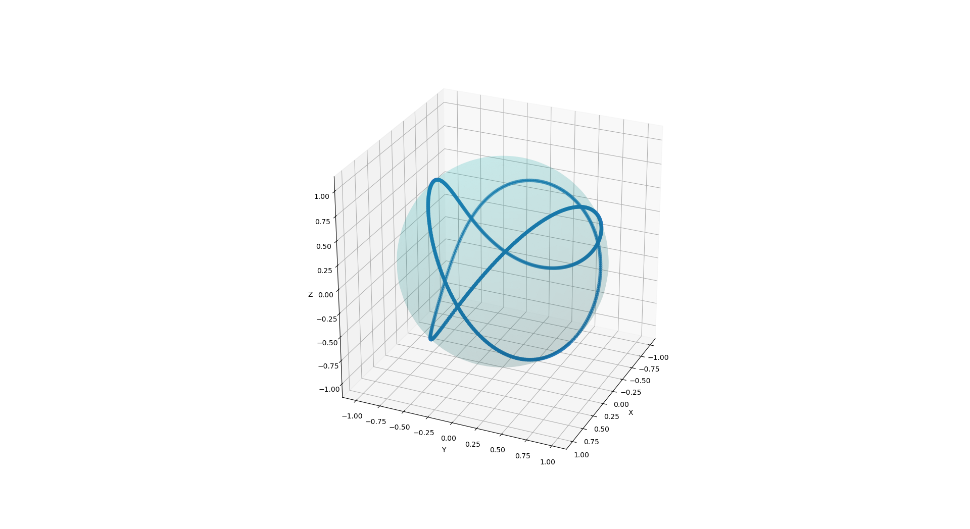
This can be seen using other shapes also. The interested reader can read this website.

Progress

I haven’t updated this website for several days as I was busy figuring out how to plot the shape sphere, as well as reading the theoretical details. I feel like the math I worked out last week is sometimes too tedious, and the longer the calculation the less interesting it becomes (loss of intuition). Regardless, I will try to classify the orbits of planet influenced by a Fixed Center in the coming days.

Credits

This post is based on the paper “A remarkable periodic solution of the three-body problem in the case of equal masses”.

I would like to again thank Dr Jenni Smillie for her guidance and support duing this project.